
Chi-square test
Published:
This tutorial employs the Null Hypothesis Significance Testing (NHST) framework and the Chi-Square ($\chi^2$) test to analyze categorical data. This approach is an alternative, yet equivalent, method to the two-sample proportion test for categorical data when a large sample size is assumed.
We are analyzing the efficacy of a vaccine against Bovine Respiratory Disease (BRD). Our data is presented in a contingency table, which is a convenient way to display categorical data where rows and columns represent different categories of two categorical variables.
1. Observed Counts ($O$): BRD Vaccine Trial Data
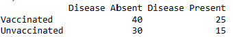
The data, supplied row-wise (Vaccinated, then Unvaccinated; Disease Absent, then Disease Present), forms the Observed Counts table:
| Disease Absent | Disease Present | Row Total | |
|---|---|---|---|
| Vaccinated | 40 | 25 | 65 |
| Unvaccinated | 30 | 15 | 45 |
| Column Total | 70 | 40 | Grand Total (N=110) |
2. Fundamental Assumptions of the Test
The $\chi^2$ test requires several assumptions to produce reliable results. In the context of this trial:
Clear and Mutually Exclusive Categories: It must be assumed that the categories (Vaccinated/Unvaccinated and Absent/Present) are clear and mutually exclusive. This ensures that one animal contributes to exactly one cell in the table.
Random and Independent Sample: The data must be collected via a random sample for both groups. This means the data must be independent, ensuring that one animal’s outcome cannot influence the outcome of another.
Large Sample Size: The test assumes a large sample size in both groups to produce reliable results. The rule of thumb for this requirement is that most of the expected counts should be greater than five.
3. The NHST Framework and Hypotheses
The NHST framework requires defining the parameter of interest and stating the null hypothesis ($H_0$).
Parameter of Interest: Since the event (disease resolution or absence) is considered random, the parameter of interest is the probability that the outcome will happen. This probability is conditioned on the treatment group. We want to see if the treatment group has a higher probability of disease absence compared to the placebo group.
The Null Hypothesis ($H_0$): Since the $\chi^2$ test is often referred to as the $\chi^2$ test of independence, the null hypothesis is that the outcome (Disease Status) is independent of the treatment group (Vaccination Status). If $H_0$ is true, the distribution of the outcome does not change no matter which treatment group it is conditioned on.
Alternative Hypothesis ($H_A$): The outcome is dependent on (or contingent on) the treatment group.
4. Calculation of Test Statistic and Null Distribution
To construct the test statistic, we must quantify the difference between our observed data ($O$) and the expected data ($E$) if $H_0$ were true.
A. Calculating Expected Counts ($E$)
We calculate the expected counts purely based on the row and column margins.
\[E = \frac{\text{Row Margin} \times \text{Column Margin}}{\text{Grand Total}}\]| Cell ($O$) | Calculation | Expected Count ($E$) |
|---|---|---|
| Vaccinated, Absent (40) | $(65 \times 70) / 110$ | 41.36 |
| Vaccinated, Present (25) | $(65 \times 40) / 110$ | 23.64 |
| Unvaccinated, Absent (30) | $(45 \times 70) / 110$ | 28.64 |
| Unvaccinated, Present (15) | $(45 \times 40) / 110$ | 16.36 |
(Assumption Check: Since all expected counts are greater than five, the large sample size assumption is met).
B. Calculating the Chi-Square Statistic ($X^2$)
We use the information from both tables to construct the test statistic, proposed by Carl Pearson. This involves taking the difference between what was observed and what was expected, squaring the difference, and dividing by the expected count to standardize the scale. This is done for all cells and then summed:
\[\mathbf{X^2} = \sum \frac{(O-E)^2}{E}\]Cell (Vaccinated, Absent): $\frac{(40 - 41.36)^2}{41.36} \approx 0.045$
Cell (Vaccinated, Present): $\frac{(25 - 23.64)^2}{23.64} \approx 0.078$
Cell (Unvaccinated, Absent): $\frac{(30 - 28.64)^2}{28.64} \approx 0.065$
Cell (Unvaccinated, Present): $\frac{(15 - 16.36)^2}{16.36} \approx 0.113$
C. Null Distribution and Degrees of Freedom (DF)
The test statistic follows the Chi-Square distribution under the null hypothesis. The constraints of the contingency table reduce the degrees of freedom (DF), which is the parameter for the $\chi^2$ distribution. Despite summing four components, a 2x2 contingency table (like ours) results in a $\chi^2$ distribution with only one degree of freedom.
5. R Code Application and Results
The function that implements the Chi-Square test in R is the chisq.test function. We supply the data in the form of a matrix, which better fits the form of a contingency table.
Step 1: Generating the Contingency Table in R
We use the matrix function. Since our data is supplied row-wise, we set the byrow argument to TRUE.
# 1. Define the counts in a vector (reading across rows: Vax/Absent, Vax/Present, Unvax/Absent, Unvax/Present)
data_counts <- c(40, 25, 30, 15)

# 2. Create the 2x2 matrix, ensuring the data is filled by row
# The Matrix function takes in a vector.
BRD_table <- matrix(data_counts, nrow = 2, ncol = 2, byrow = TRUE)

# 3. Add descriptive names for clarity
rownames(BRD_table) <- c("Vaccinated", "Unvaccinated")
colnames(BRD_table) <- c("Disease Absent", "Disease Present")

# Display the resulting matrix
print(BRD_table)
Step 2 : Running the Chi-Square Test
# Pass the matrix to the test function
chisq_result <- chisq.test(BRD_table, correct = FALSE) # Setting correct=FALSE ensures we match the Pearson standard formula without continuity correction

# Display the test results
print(chisq_result)

Step 6: Conclusion
The results of the hypothesis test are : | Component | Value | |——————————-|——–:| | Chi-Square Statistic (X²) | 0.301 | | Degrees of Freedom (df) | 1 | | P-value | 0.583 |
f we use a standard significance level of 5% ($\alpha = 0.05$), we compare the P-value (0.583) to this threshold. Since the P-value (0.583) is greater than 0.05, we fail to reject the null hypothesis.We conclude that there is not sufficient statistical evidence to suggest that the outcome (BRD status) is dependent on (or contingent on) the vaccination status